Survival analysis. Less code. Not less statistics.
Run the complete workflow in your browser

Wait for Ready, run the data setup once, then open either analysis tab. Run the code blocks in that tab from top to bottom. The first run can take a moment while R and the packages start.
The package uses flextable by default for document-ready output. This browser demo uses format = "gt" so the tables display here. Use RStudio for the full flextable and export experience.
Understand the teaching data
The teaching dataset contains 137 people enrolled in a Veterans Administration lung-cancer treatment trial. It is included with gtregression and is intended for demonstrating time-to-event methods.
| Variable | What it records | Coding or unit |
|---|---|---|
trt |
Randomised treatment group | 1 = standard; 2 = test |
celltype |
Histological cell type | Squamous, small-cell, adeno or large-cell |
time |
Follow-up time | Days |
status |
Event indicator | 1 = death observed; 0 = censored |
karno |
Karnofsky performance score | Higher scores indicate better functional status |
diagtime |
Time from diagnosis to study entry | Months |
age |
Age at study entry | Years |
prior |
Previous therapy | 0 = no; 10 = yes |
An event is the outcome of interest. A censored observation means the event was not observed during the available follow-up; it does not necessarily mean the person remained event-free forever.
1. Summarise survival before modelling
Begin with the denominator, number of observed events, censoring and median survival in each treatment group.
2. Draw the Kaplan–Meier curves
The result is a ggplot object, so every element—titles, axes, colours, annotations, themes and dimensions—is completely customisable.
3. Fit separate crude Cox models
cox_reg() fits the same model structure for each exposure and reports hazard ratios consistently—without constructing a Surv() formula.
Exposure levels, reference groups and labels are aligned automatically. They remain easy to relabel and customise for a manuscript or report.
4. Fit one multivariable Cox model
Set multivariable = TRUE to fit one mutually adjusted model. Use adjust_for = when selected exposures require a defined adjustment set rather than adjustment for every variable.
5. Merge the crude and adjusted tables
Regression tables merge in a single command. The resulting tables are fully customisable as flextable or gt outputs; this browser demonstration uses gt, while flextable remains the package default.
6. Compare the estimates visually
This is also a ggplot output: resize it, restyle it or add annotations using the familiar ggplot2 workflow.
7. Build a publication-style forest plot
The same fitted objects can be passed to forest_reg(). The output below was rendered in desktop R so the full table-style forest plot fits the page.
cox_forest_data <- forest_df(
  uni = cox_crude,
  multi = cox_adjusted
)

cox_forest <- forest_reg(
  df = cox_forest_data,
  effects = c("Crude HR", "Adjusted HR"),
  ticks_at = c(0.5, 1, 2, 4)
)

save_forest(cox_forest, "cox-forest", format = "png")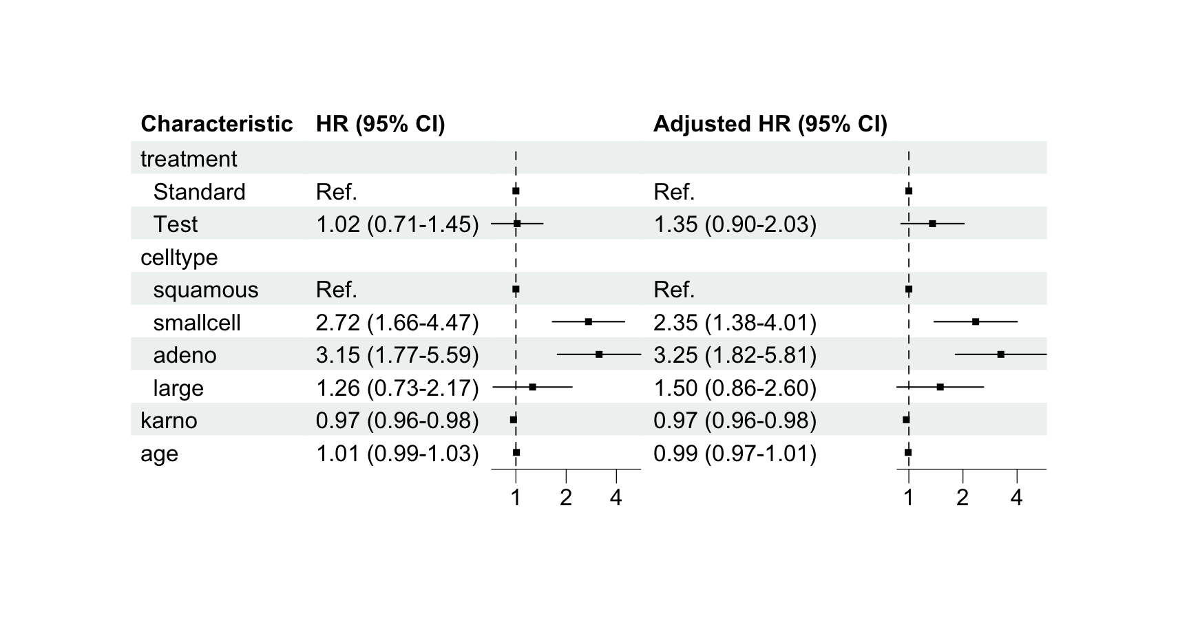
This is a pre-rendered output because a browser-based WebR session has limitations when laying out the complete figure. forest_reg() addresses a visual audience while retaining the effect size and 95% confidence interval. It produces the kind of self-contained figure that works particularly well in journal submissions, reports and presentations.
8. Check the proportional-hazards assumption
Parametric models describe survival using an assumed distribution and can report time ratios. A time ratio above 1 suggests longer survival time; below 1 suggests shorter survival time, conditional on the selected model.
1. Compare candidate distributions
Candidate distributions are compared in one call, providing a consistent starting point for selecting a parametric model.
2. Compare observed and fitted survival
The fitted survival curves are ggplot outputs and remain completely customisable.
3. Fit separate log-logistic models
Exposure levels, reference groups and labels are aligned automatically and can be customised without rebuilding the table.
4. Fit one multivariable parametric model
Set multivariable = TRUE for one mutually adjusted parametric model, or use adjust_for = to define selected adjustment sets for particular exposures.
5. Merge crude and adjusted time ratios
Crude and adjusted time-ratio tables merge in one command. The output remains entirely customisable as a flextable or gt table.
6. Compare the time ratios visually
The combined regression figure is a ggplot output and can be restyled, annotated and exported at the dimensions required by a journal.
7. Produce the parametric forest plot
parametric_forest_data <- forest_df(
  uni = parametric_crude,
  multi = parametric_adjusted
)

parametric_forest <- forest_reg(
  df = parametric_forest_data,
  effects = c("Crude time ratio", "Adjusted time ratio"),
  ticks_at = c(0.25, 0.5, 1, 2)
)

save_forest(parametric_forest, "parametric-forest", format = "png")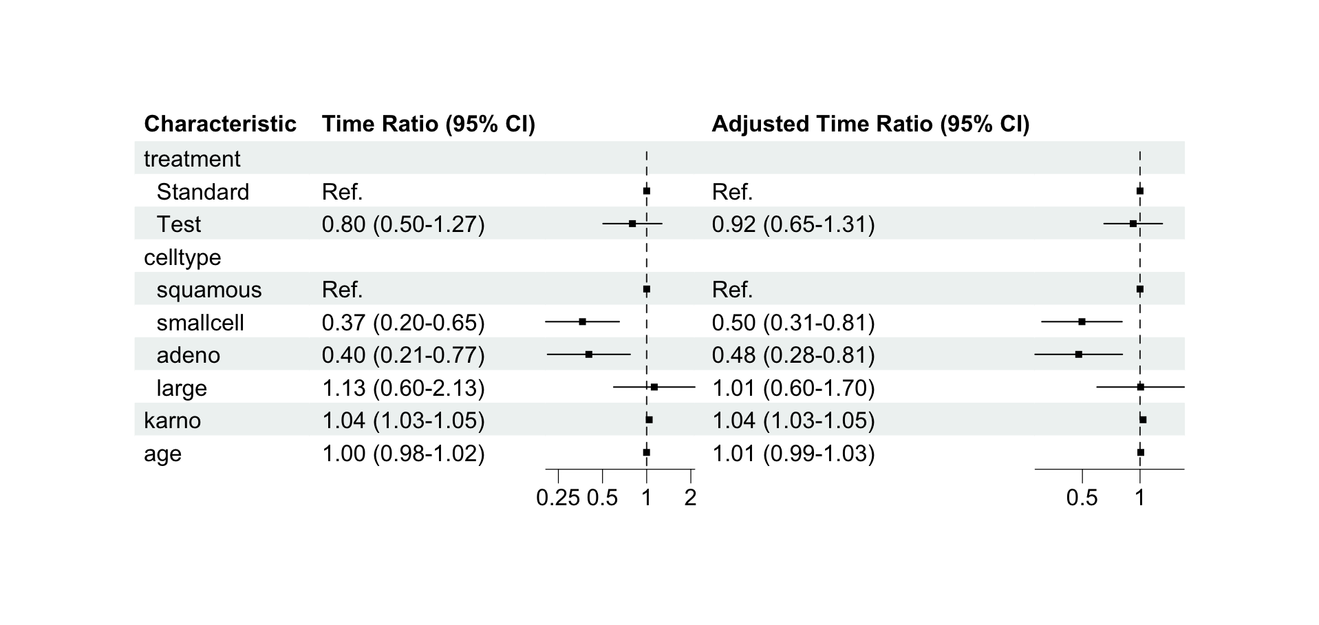
This pre-rendered figure avoids the layout limitations of the WebR browser. It combines effect sizes, 95% confidence intervals and the graphical display in one publication-ready output for readers who absorb results visually.
One package, two survival frameworks
Cox: Kaplan–Meier context → Crude HRs → Adjusted HRs → Merged table → Forest plot → PH diagnostic
Parametric: Compare distributions → Inspect fitted curves → Crude time ratios → Adjusted time ratios → Merged table → Forest plot
gtregression does not replace careful model specification, clinical reasoning or interpretation. It gives those decisions a consistent, reproducible and publication-ready workflow.
Cite gtregression
Polani R, Eliyas S, Sakthivel M, Kaviprawin M, Krishnamoorthy Y, Majella M (2026). gtregression: Tools for Creating Publication-Ready Regression Tables. R package version 1.1.0. doi:10.32614/CRAN.package.gtregression
In R, run citation("gtregression") to retrieve the current citation and BibTeX entry.